Abderrahim Belissaoui, Application Engineer, CES – Dubai, UAE.
In this blog post, I delve into the concept of compressed sensing and its applications in array signal processing, demonstrating its effectiveness through MATLAB implementations.
Compressed sensing offers significant advantages over traditional Direction-of-Arrival (DOA) estimation techniques such as Multiple Signal Classification (MUSIC) and Estimation of Signal Parameters via Rotational Invariance Technique (ESPRIT) algorithms particularly in its ability to accurately recover signals from a limited number of measurements. This approach not only enhances computational efficiency but also improves performance in scenarios with sparse data, making it a powerful tool in modern signal processing.
introduction
Compressed Sensing (CS) has emerged as a result of the challenges in efficiently acquiring and reconstructing signals in modern signal processing. CS is a revolutionary technique that allows signals to be reconstructed from fewer samples than traditional methods. It leverages the sparsity feature of signals to optimize data acquisition, making it particularly useful in applications where data collection is expensive or constrained by hardware limitations.
Compressed sensing has a wide range of applications, including medical imaging, wireless communications, and radar systems. It provides advantages such as reduced data storage, faster processing speeds, and improved accuracy in reconstructing high-dimensional signals.
An area where CS can make improvements is array signal processing, for instance, CS can be used for estimating the Direction of Arrival (DOA) of signals. Traditional DoA estimation techniques, including multiresolution algorithms, rely on large antenna arrays and high sampling rates, which can be impractical in real-world scenarios. CS-based approaches, on the other hand, exploit the sparsity of directions to reduce the number of required measurements while maintaining accurate estimation.
background
Compressed Sensing Problem
The matrix models the linear measurement (information) process . Then one tries to recover the vector by solving the above linear system. Traditional theorem suggests that the number m of measurements, i.e., the amount of measured data, must be at least as large as the signal length N (the number of elements of x). Current technology is all based around this principle, in particular for analog-to-digital conversion (medical imaging, radar, and mobile communication also rely on this principle). Indeed, If m < N, then classical linear algebra indicates that the linear system is underdetermined and that there are infinite solutions. In other words, without additional information, it is impossible to recover x from y in the case m < N. This is also applicable to the Shannon sampling theorem, which indicates that the sampling rate of a continuous-time signal must be twice its highest frequency to ensure reconstruction. In scenarios where the available data is insufficient for direct signal reconstruction, compressed sensing, combined with a recovery algorithm, can still accurately reconstruct the original signal—provided it exhibits sparsity in at least one domain, such as time, frequency, or space.
sparsity
A signal is defined as sparse if most of its components are zero. As empirically observed, many real-world signals are compressible because they are well approximated by sparse signals—often after an appropriate change of basis. For example, an ideal sine wave in the frequency domain corresponds to a single frequency component. This is represented as a single peak (or two symmetric peaks for real signals) in the frequency spectrum. Using MATLAB, let’s see if a double-tone signal is sparse in any domain.

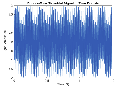
The double-tone signal is clearly non-sparse in the time domain. Nevertheless, this signal could be sparse in the frequency domain. Let’s check this in MATLAB.

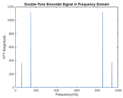
Plotting the computed spectrum shows sparsity of the signal in the frequency domain. Sparsity as explained before can be quantified by the number of non-zero elements of the signal in the analysis domain.

The percentage of non-zero elements in the double-tone sinusoidal signal is 0.266667.
Compressive Sensing Recovery Algorithms
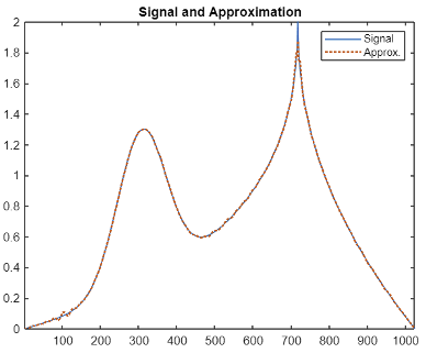
One of the key aspect of compressive sensing is the need for efficient reconstruction algorithms to reconstruct a sparse signal from a limited number of measurements. The reconstruction of compressed sampled signal involves finding solution of an underdetermined system of linear equations and therefore has infinite solutions. The basic sensing equation is given by Eq 1.
The signal reconstruction process is essentially to find the best estimate of the original signal from all the possible solutions obtained from solving Eq 1. This is essentially a minimization problem.
The L1-minimization problems in CS signal reconstruction are usually solved using convex optimization methods. In addition, there exist greedy methods for sparse signal recovery which allow faster computation compared to L1-minimization. Some of these algorithms are:
- Matching Pursuit (MP)
- Orthogonal Matching Pursuit (OMP)
- Compressive Sampling Matching Pursuit (CoSaMP)
- Iterative Hard Thresholding Algorithm (IHTA)
The following MATLAB example shows how to reconstruct a signal using OMP algorithm.

Sparse Arrays and DoA Estimation
What are Sensor Arrays?
Sensor Arrays are collections of antennas, microphones, or acoustic transducers arranged in a pattern. Arrays convert signals into radiated energy for transmission to a target. Sensor arrays also convert incoming energy from a source or reflecting object into signals. The performance of arrays in many ways exceeds that of the individual array elements. A specific type of arrays is phased array that has three main advantages over individual elements:
- Improved spatial resolution — view more detailed resolution when localizing and imaging a target.
- Electronic steering — use an array steering vector to increase detection performance in any direction.
- Interference suppression — enable advanced interference suppression, including jammer nullification, adaptive beamforming, and high-resolution direction finding.
What are Sparse Arrays?
Sparse arrays have recently attracted considerable attention for their application in improving active and passive sensing in radar, navigation, underwater acoustics and wireless communications. Sparse array signal processing provides a systematic framework for sparse sampling and array structure with enlarged aperture, enhanced spatial resolution, increased degrees of freedom (DOFs) and reduced mutual coupling. Commonly used sparse arrays include:
Minimum Redundancy Array
one of the earliest sparse array designs is minimum redundancy array (MRA). An MRA is designed to provide maximum resolution for a given number of elements in the array. The idea behind an MRA is to use true elements to measure the phase difference with unique element spacing. The figure below displays MRA Array:

Nested Arrays
Recently, nested arrays and coprime arrays have become popular choices for sparse arrays, as the identification of an MRA can be difficult and not readily available.

Coprime Arrays:
The idea of a coprime array is to form the array with two sub-arrays whose element spacings are coprime to each other. The issue with a nested array is that it contains a dense array, making it more prone to mutual coupling effects between array elements. A coprime array is easy to construct and on average it places elements further apart, thus alleviating the mutual coupling effects.

To estimate Direction-of-Arrival using these sparse arrays, full arrays must be reconstructed first. Once we obtain the full array, we can just apply any known DOA estimation algorithm like MUSIC or ESPRIT to the reconstructed signal measurements.
DoA Estimation Using Compressed Sensing
In general, in a DOA estimation scenario, the number of incoming directions is far less than the number of elements. Therefore, the problem is sparse. In addition, trying to identify these directions from a single snapshot also makes the problem underdetermined. Compressive sensing techniques are well-suited to address these challenges. The following case study demonstrates the use of an OMP CS recovery algorithm to estimate DoA using a coprime array:
- Build and Visualize a Coprime Array Architecture

2. Array Reconstruction

3. Compute and Plot Beamscan Spectrum


4. Direction of arrival estimation using Compressed Sensing


conclusion
This blog explored compressive sensing for a common array signal processing application: direction of arrival (DOA) estimation. It highlighted the role of sparsity and recovery algorithms in accurately reconstructing incoming signal directions using a sparse array and fewer measurements. The implementations demonstrated how signals can be efficiently recovered, enhancing estimation accuracy while reducing computational complexity. These techniques offer a strong foundation for further research, optimization, and real-world applications in fields like radar, communications, and sensor networks.