Simulink R2022a: The new release of Matlab R2022a is out with new products and plenty of updates. In this video Vishwa Samba will show you how to use local solvers in Simulink simulations; a new feature available in R2022a.
We all know that Simulink models are solved with a single solver, and sometimes if the subcomponents of the model have different dynamics, then one solver might not fit the whole model. The accuracy of the simulation may vary or the time required for the simulation has increased.
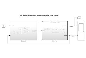
 To overcome this problem, we can use “local solvers” in Simulink Simulations. Using the example of DC motors. A DC motor has mechanical and electrical subsystems. The time constant for a mechanical subsystem is more than the electrical subsystem.
If one solver is used for simulation, then the step size required will be small enough to catch the electrical time constant. Therefore, the simulation time will increase. To reduce the simulation time needed, we can use a local solver for the mechanical subsystem.
Simulink R2022a
With the help of local solvers we can speed up simulation by using an inexpensive solver on a subset of the model. An inexpensive solver could be a lower-order solver, for example, using an “ode1 solver” instead of an “ode3”, or just by using a solver with a larger step size.
The choice of solver and step size represents a tradeoff between computational cost and accuracy. A local solver allows you to fine-tune this tradeoff for different subsections of the model.
More information on the latest release MATLAB 2022a and other release highlights
To overcome this problem, we can use “local solvers” in Simulink Simulations. Using the example of DC motors. A DC motor has mechanical and electrical subsystems. The time constant for a mechanical subsystem is more than the electrical subsystem.
If one solver is used for simulation, then the step size required will be small enough to catch the electrical time constant. Therefore, the simulation time will increase. To reduce the simulation time needed, we can use a local solver for the mechanical subsystem.
Simulink R2022a
With the help of local solvers we can speed up simulation by using an inexpensive solver on a subset of the model. An inexpensive solver could be a lower-order solver, for example, using an “ode1 solver” instead of an “ode3”, or just by using a solver with a larger step size.
The choice of solver and step size represents a tradeoff between computational cost and accuracy. A local solver allows you to fine-tune this tradeoff for different subsections of the model.
More information on the latest release MATLAB 2022a and other release highlights